Details

Forging the future of Geological Mapping with ML

Date: June 29th 2022

Project Lead:

Hazen Russell | Lead Sedimentologist GS

Nicolas Benoit | Lead Hydrogeologist, GSC

William Parkinson | Lead Technical Product Manager, EarthDaily Analytics

Participants:

Afshin Amini (Researcher at UBC)

Debjani Mukherjee(Consultant Green Connect Solutions Inc)

Hazen Russel– Overview of the project

Surficial geological mapping comprises of photographs, stereoscope, and a cognitive ability of the interpreter. The challenge is to replace all 3 of those with an array of digital data from remote sensing, digital elevation models and potentially other data sets. Deploy Machine learning for the cognitive functions and bring all that together and see how it works. We chose a location in northern Saskatchewan with available geological mapping, also providing the training dataset.

Nicolas Benoit:

There are multiple challenges in application of machine learning to the surficial geological mapping. Besides the challenge of computing resource, what we see on the surface is not necessarily same as what we find below the surface. So, it is difficult to find features that are correlated to that kind of geological unit. Also, in geology spatial distribution of the units are often non-stationary. So, there can be area with different proportion of different units. The proportions can be very high for one unit and very different for another. Reproducing these small features is easier with images than tabular algorithm. Validation of the data, making sure that the data set is good and well correlated to the units poses another challenge. It is important to clean the data prior to application of machine learning, which we may not have done very well. It is hard to get more informative data like derivative data from common data - topography map or map of erodibility etc.

Debjani Mukherjee:

I was unable to read the data set or continue data wrangling with my computer. I tried to figure out few utilities with support from project lead, Nicolas- increasing RAM, loading data through API, use of GPU and finally subscribed google pro and yet my computer crashed. Nicolas created a sample data set for me. I followed up by EDA, changing the data types and splitting into train and test dataset. Selected few features and then used XGboost to fit the data, selected parameters using hyper parameters like GridSearchCV. The Gradient Boost classification was executed only with 3 estimators. Some of the other operations included – Random Forest classification, PCA transformation, LLE, MDH, F1 score – 0.87, positives and negatives were not close in the scatter plots, so it was hard to classify.

Although I was unable to come up with a working model, but it had been a very rewarding experience working with Hazen, Nicholas, William and Afshin. This is the first time I worked with geospatial data set, and the extremely helpful team created an amazing learning experience for me.

Afshin Amini:

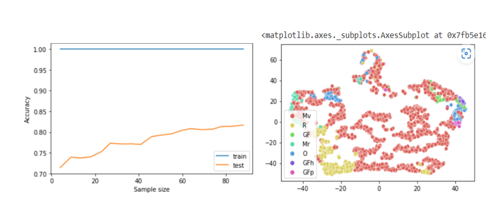
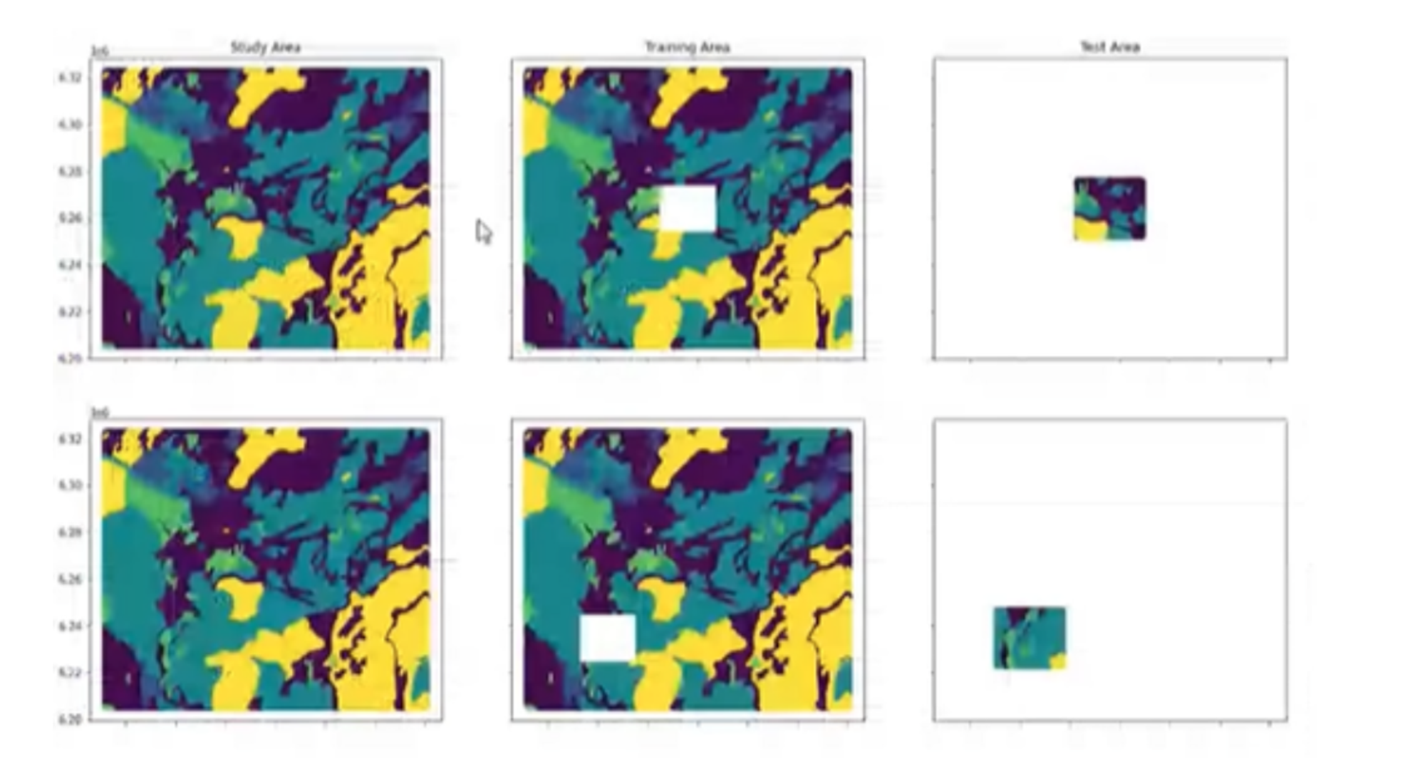
It was interesting to work with the open-ended aspect of the project. The dataset consists of 220 features and 1.9 million data samples. So, it is a huge dataset. Database has some nans or missing values. There are 13 labels or classes that we were trying to predict. There are some classes which are highly under-represented. Some classes contribute only 1% of the data. The subgroups were merged with more general groups for the classes which were somehow related, resulting in 5 major classes. This allowed easier handling of data. The mapping area was divided into 5 basic models. At first a tile was removed from the middle and the surrounding area was used to train the model and try to predict.

Next the location of the tile was changed through out the model to see how the performance of the model changed depending on where we were trying to predict. As the number of features were very high, running the models took very long time. Also, I had run random forest classifier and f1 score was 72%. Some features contributed more to the prediction than the rest. Therefore, features contributing more than 10% totalling 54 out of 220 were used for the analysis. This reduced the size of the dataset. The same exercise was repeated for all the 5 areas based on the locations where the tile was moved. F1 score varied from 71% to 85% accuracy. This proved that the models were very sensitive to the location.

Next step: Analyze permutated feature importance, partial dependence plus and ice plots. Alternative approach could be treating the under-represented classes for anomaly detection, and train models to specifically pick up these classes. Objective is to identify those features which were contributing to the low precision and recall values and finally improve the F1 score.

William Parkinson: Final comments

Afshin’s models are returning spatially correlated predictions, which fits the geologic structures. The spatial correlation is core of the challenge. There may be inconsistency in the results but the regions are identified well which is correlating the truth. As mentioned earlier by Nicholas, the features that are interpreted using stereo photos, are essentially an interesting combination of what we understand about processes or what we see on the surface or what we understand about topography and how all those are brought together for some sort of interpretation. So, it’s much more complicated than a feature extraction problem which neural nets do at their best.

Recommendation for Afshin: To improve the accuracy of the under-represented classes, include other classified results as input to those classes. Example- Certain surface geologic features are likely to occur adjacent to other ones. So, a piece wise classification may help to improve the F1 score.

Recommendation for Debjani: Gather a deeper understanding of correlated components within the PCA by looking at the weightings in the PCA